
Overview of the Course
This course provides a comprehensive exploration of Next-Generation Sequencing (NGS), an advanced and transformative technology in genomics. It is designed to guide learners through the historical evolution, technical foundations, data processing methodologies, and broad applications of NGS, equipping them with a robust understanding of both theoretical concepts and practical tools.
Introduction to NGS
The course begins with an Introduction, presenting an overview of NGS and tracing its evolution from early sequencing methods to modern platforms. This section establishes the groundwork for understanding the rapid advancements and adoption of NGS across diverse biological and medical fields.
- NGS History: Learn about the milestones and breakthroughs that shaped NGS as a revolutionary tool in genomics.
Data Generation
The Data Generation module delves into the mechanics of how sequencing data is created. It includes insights into read generation, error rates, read lengths, and the importance of coverage and depth in sequencing experiments.
Data Processing Concepts
A critical aspect of the course focuses on Data Processing Concepts, which are foundational to extracting meaningful insights from raw sequencing data.
- Quality Control: Techniques to assess and ensure high-quality sequencing data.
- Reads Alignment: Methods to align sequencing reads to reference genomes.
- File Formats: Explore standard file formats like FASTQ, BAM, and VCF used in NGS workflows.
Variant Detection
The Variant Detection module covers the identification of genetic variants from sequencing data. This section includes a breakdown of variant types, calling methodologies, statistical models, and challenges in detection.
- Variant Calling Pipelines: Detailed discussions on popular frameworks, including:
- GATK pipeline
- Nf-core pipelines
- Bcbio pipelines
- Population Genomics: Investigate the implications of variant detection on population studies.
Functional Annotation
The Functional Annotation module focuses on interpreting the biological and clinical significance of identified variants. This section introduces tools and frameworks for functional annotation and examines the ethical dimensions of genomic analysis.
- Annotation Tools: Tools like ANNOVAR and Ensembl Variant Effect Predictor (VEP).
- Clinical Interpretation: Methods for translating genomic data into clinical insights.
- Ethical Considerations: Discussion on privacy, data sharing, and consent.
NGS Applications
The course concludes with a comprehensive overview of the Applications of NGS across various domains, demonstrating the transformative potential of sequencing in modern science and medicine.
- Disease Research: Role of NGS in understanding and addressing genetic disorders.
- Personalized Medicine: Insights into tailoring treatments based on individual genomic profiles.
- Evolutionary Genomics: Exploring evolutionary relationships and history through sequencing.
- Metagenomics and Multi-Omics: Broad applications in studying microbiomes and integrating multi-dimensional biological data.
Learning Outcomes
By the end of this course, learners will be equipped to:
- Understand the technical principles and challenges of NGS.
- Analyze sequencing data with appropriate tools and workflows.
- Detect and annotate genetic variants with accuracy.
- Apply NGS to real-world problems in genomics, medicine, and beyond.
- Address ethical considerations in the use of sequencing technologies.
This course is suitable for researchers, clinicians, and professionals seeking a deep dive into NGS technologies, their applications, and the broader impact of genomics in shaping science and healthcare.
Disclaimer: A portion of the content in this course has been generated with the assistance of artificial intelligence. While every effort has been made to ensure accuracy and quality, the use of AI-generated material may result in occasional limitations or errors. We encourage learners to critically assess the information presented and seek additional resources as needed.
A Brief History and Evolution of Sequencing Technologies: From First to Third Generation
The sequencing of DNA has revolutionized fields like genomics, medicine, and biology. Since the first DNA sequencing methods were developed, advances in technology have led to faster, cheaper, and more accurate ways of reading the genetic code.
First Generation Sequencing: Sanger Sequencing (1977)
The first successful DNA sequencing method was developed by Frederick Sanger in 1977. This method, called Sanger sequencing or dideoxy sequencing, became the foundation of modern genetics. It relies on selective incorporation of chain-terminating dideoxynucleotides during DNA replication, which are labeled either radioactively or with fluorescent dyes.
-
Key Features:
- High accuracy: Sanger sequencing is highly accurate for short to medium DNA sequences (up to 1000 base pairs).
- Laborious and slow: Despite its accuracy, Sanger sequencing is time-consuming and requires significant manual effort.
- Costly: As the genome size increases, Sanger sequencing becomes prohibitively expensive.
- Impact: The method enabled the sequencing of small genomes, like that of viruses and bacteria, and later played a pivotal role in sequencing the human genome in the early phases of the Human Genome Project.
Second Generation Sequencing (Next-Generation Sequencing, NGS)
The need for faster and more scalable sequencing methods drove the development of next-generation sequencing (NGS), also known as second-generation sequencing, in the mid-2000s. This generation introduced massively parallel sequencing, enabling millions of DNA fragments to be sequenced simultaneously.Second-generation technologies revolutionized genomics by making whole-genome sequencing (WGS) more accessible and affordable. These technologies have enabled large-scale projects such as the 1000 Genomes Project and have applications in personalized medicine, cancer research, and rare disease diagnosis.
Key Technologies:
-
Illumina Sequencing:
-
Working Principle: Illumina technology uses reversible terminator chemistry, where nucleotides are fluorescently labeled. Each incorporated nucleotide emits a unique signal, which is recorded in real-time.
-
Advantages: Highly scalable, cost-effective, and capable of producing high-throughput data (up to billions of reads).
-
Limitations: Short read lengths (typically 50–300 bp), which can complicate the assembly of large genomes. Roche 454.
-
-
Pyrosequencing:
-
Working Principle: Pyrosequencing is based on detecting the release of pyrophosphate when a nucleotide is incorporated.
-
Advantages: Longer reads than Illumina (up to 1000 bp).
-
Limitations: Higher costs and lower throughput compared to Illumina, leading to its decline in popularity.
-
-
SOLiD Sequencing:
-
Working Principle: SOLiD uses ligation-based sequencing, where fluorescently labeled oligonucleotides hybridize to the template.
-
Advantages: High accuracy due to error correction with two-base encoding.
-
Limitations: Lower throughput than Illumina, shorter read lengths.
-
Third Generation Sequencing: Single-Molecule Real-Time (SMRT) and Nanopore Sequencing
Third-generation sequencing technologies represent the latest advancements, focusing on reading long stretches of DNA and sequencing in real-time without the need for amplification. This addresses the limitations of second-generation technologies, particularly in terms of read length and sample preparation. These technologies are ideal for de novo genome assembly, structural variant detection, and metagenomics. Their ability to sequence long, unfragmented DNA molecules has opened new possibilities in understanding complex regions of the genome, including repetitive sequences and large structural variants. These technologies are also being employed in clinical settings for rapid pathogen detection and in field-based genomics due to the portability of devices like Oxford Nanopore's MinION.
Key Technologies:
-
Pacific Biosciences (PacBio) Single-Molecule Real-Time (SMRT) Sequencing:
-
Working Principle: SMRT sequencing captures real-time nucleotide incorporation by DNA polymerase as it synthesizes DNA. It can read entire DNA molecules without the need for fragmentation.
-
Advantages: Extremely long reads (up to 100 kb), high accuracy (especially with circular consensus sequencing), and ability to detect epigenetic modifications.
-
Limitations: Higher error rates compared to NGS in early versions, though newer systems have improved accuracy.
-
-
Oxford Nanopore Sequencing:
-
Working Principle: Nanopore sequencing uses biological nanopores to detect changes in ionic current as DNA or RNA passes through, allowing direct reading of nucleotide sequences.
-
Advantages: Ultra-long reads (potentially up to 2 Mb), portability (MinION sequencer), and real-time data output. It can also sequence RNA and detect base modifications directly.
-
Limitations: Higher error rates compared to Illumina, although accuracy is improving with advanced models.
-
Future Directions and Implications
The evolution of sequencing technologies continues to push the boundaries of genomic research. As third-generation technologies mature and costs decrease, the possibility of true personalized genomics comes closer to reality. Future advances may include higher accuracy, longer reads, and greater affordability, ultimately enabling routine clinical use for precision medicine, agricultural genomics, and global biodiversity efforts. Additionally, the integration of artificial intelligence and machine learning in data analysis, alongside improvements in bioinformatics tools, will further enhance the interpretation of large-scale genomic data, contributing to the discovery of novel therapies and deeper understanding of biological systems. In conclusion, from the labor-intensive days of Sanger sequencing to the high-throughput capabilities of NGS and the innovative third-generation technologies, DNA sequencing has come a long way. Each generation has contributed to a deeper understanding of genetics and biology, paving the way for transformative applications in medicine, agriculture, and evolutionary studies. As we look to the future, the continued evolution of sequencing technologies promises to unlock even more of the mysteries hidden within the genetic code.
- Ressource 1: Source 1 : Next-generation sequencing technologies: An overview .
- Ressource 2: Source 2 : Overview of Next Generation Sequencing Technologies .
Generating Raw Sequencing Reads
The generation of raw sequencing reads serves as an essential foundation in genomics and bioinformatics research. It involves the process of converting DNA or RNA from a biological sample into a digital format for subsequent analysis. The unprocessed sequencing reads serve as the basis for nearly all future analyses, including genome assembly, variation identification, and gene expression investigations. High-throughput sequencing technologies have revolutionized the field by allowing for the rapid and cost-effective generation of massive amounts of sequencing data. These raw reads contain valuable information about the genetic makeup of an organism, providing researchers with a wealth of data to explore and analyze.
1. Sample Preparation: DNA/RNA Extraction
The process starts with sample preparation, during which DNA or RNA is extracted from a biological source, such as blood, tissue, or cells. The quality of the extracted material is paramount, as damaged or contaminated samples can result in suboptimal sequencing outputs.
-
DNA Extraction: High-quality genomic DNA is obtained for genomic investigations utilizing various techniques and kits specifically developed for purifying DNA from biological materials.
-
RNA Extraction: In transcriptomics or RNA sequencing (RNA-seq), RNA is isolated from the sample. Maintaining RNA integrity is essential due to its greater susceptibility to degradation compared to DNA.
Upon purification, the nucleic acids undergo quality assessments to verify their concentration and purity prior to advancing to subsequent processes.
2. Library Preparation
The initial phase of the sequencing process is library preparation, which generally encompasses the following steps:
-
Fragmentation: The isolated DNA is too large for direct sequencing, so it is cleaved into smaller fragments using mechanical (e.g., sonication) or enzymatic methods.
-
Adapter Ligation: Short, synthetic DNA sequences known as adapters are ligated to the termini of each DNA fragment. These adapters comprise sequences recognized by the sequencing platform.
-
Barcode Addition: Distinct barcodes (short DNA sequences) are incorporated to differentiate samples during the pooling of many specimens in a single run (multiplexing).
-
Amplification (Optional): In instances of insufficient DNA quantities, the fragments may be amplified via PCR to guarantee adequate material for sequencing. PCR-free techniques are favored where feasible to eliminate biases.
3. Sequencing: Data Generation
Upon preparation of the library, the sample proceeds to sequencing. The selection of sequencing technology is contingent upon parameters like read length specifications, accuracy, and requirements for the project. Prominent sequencing platforms include:
Illumina Sequencing
-
Technology: Illumina employs sequencing by synthesis (SBS), wherein fluorescently labeled nucleotides are integrated into an elongating DNA strand, and a camera captures the signal for base identification.
-
Short Reads: Generally generates brief reads (50–300 bp) with elevated precision.
-
Applications: Suitable for various purposes including whole-genome sequencing (WGS), RNA sequencing (RNA-seq), and exome sequencing.
-
Challenges: Short reads may encounter difficulties in resolving intricate regions, particularly those characterized by structural changes or elevated GC content.
Nanopore Sequencing
-
Technology: Nanopore sequencing, developed by Oxford Nanopore, involves the translocation of DNA or RNA via a nanopore, measuring variations in ionic current to ascertain nucleotide sequences.
-
Long Reads: Able to produce substantial read lengths (up to several megabases).
-
Applications: Beneficial for addressing structural variants, repeating sections, and generating real-time data.
-
Challenges: Elevated error rates relative to Illumina, however advancements in base-calling are mitigating these errors.
PacBio Sequencing (SMRT)
-
Technology: PacBio's Single Molecule, Real-Time (SMRT) sequencing produces longer reads with elevated precision.
-
Applications: Preferred for tasks necessitating extensive readings to construct intricate genomic regions or identify structural changes.
-
Challenges: Elevated cost per base compared to Illumina.
4. Quality Control of Raw Reads
Following the generation of raw sequencing reads, quality control (QC) is essential to guarantee data integrity and dependability for subsequent studies. This procedure often involves assessing read quality, filtering poor data, and eliminating artifacts. It is imperative that the final collection of reads maintains high quality to ensure accurate and reproducible outcomes. A dedicated section will address the particulars of quality control methods and tools.
5. Data Storage and Management
Sequencing produces extensive data that requires effective management and storage.
-
Data Formats: Raw reads are preserved in FASTQ format, encompassing both sequences and quality ratings. Compressed formats such as BAM or CRAM are utilized for long-term storage.
-
Backup: Due to the magnitude of genetic data, routine backups utilizing high-capacity storage devices are required. Cloud resources or local high-performance computing storage systems are commonly utilized.
-
Data Sharing: To facilitate reproducibility and adhere to open data standards, raw sequencing data is frequently submitted to public repositories such as the Sequence Read Archive (SRA) or the European Nucleotide Archive (ENA).
The production of raw sequencing reads is fundamental to genomics and bioinformatics. Each step, from DNA/RNA extraction and library preparation to sequencing and quality control, is essential for maintaining the accuracy of downstream analyses. With the advancement of sequencing technologies, researchers can further investigate novel realms in genomics with enhanced resolution and precision. The accessibility of raw sequencing data in public repositories facilitates transparency and reproducibility of research outcomes. Researchers can readily access and authenticate the data, fostering collaboration and further progress in the domain of genetics.

-
Resource 1: Library preparation methods for next-generation sequencing: Tone down the bias .
-
Resource 2: Zverinova, S., & Guryev, V. (2022). Variant calling: Considerations, practices, and developments. Human Mutation, 43(8), 976–985. .
Sequencing Errors and Their Causes
Sequencing errors are a common challenge in next-generation sequencing (NGS) and can affect downstream analyses, including variant calling, genome assembly, and gene expression quantification. Understanding the causes of these errors and applying quality control (QC) steps is crucial to improving data reliability.
Types of Sequencing Errors
- Substitution Errors
Occur when an incorrect base is incorporated during the sequencing process (e.g., an "A" is called as a "G"). This can happen due to signal misinterpretation, especially in regions with low-quality base calls.
- Insertion and Deletion (Indel) Errors
These errors occur when a base is incorrectly added (insertion) or omitted (deletion) in the read. Indel errors are more common in long-read sequencing platforms like PacBio and Nanopore, where signal interpretation over longer reads can become less precise.
- Homopolymer Errors
These errors happen in regions of repetitive bases, such as "AAAA" or "GGGG," where sequencing technologies may struggle to accurately determine the length of the homopolymer. This issue is especially prominent in technologies like Ion Torrent.
- Phasing and Pre-phasing Errors (Illumina)
Phasing errors occur when nucleotides in a cluster are out of sync during sequencing by synthesis (Illumina). When a strand lags (phasing) or moves ahead (pre-phasing) of the rest of the cluster, it can result in miscalled bases.
- GC-content Bias
Regions of the genome with very high or very low GC content are more likely to have errors. For example, regions with high GC content may be difficult to amplify, leading to incomplete sequencing, while low GC content may result in inefficient binding during sequencing.
- Context-specific Errors
Certain sequence contexts, such as repetitive regions or highly structured sequences (like hairpins), can lead to sequencing artifacts, especially in short-read platforms that rely on amplification.
- Chimeric Reads
Sometimes, fragments from different parts of the genome are accidentally joined during library preparation, producing reads that do not correspond to any actual sequence in the sample. These are known as chimeric reads and can lead to misalignment and false variant calls.
Causes of Sequencing Errors
-
Platform-specific Limitations
- Each sequencing technology has inherent strengths and weaknesses. For example:
- Illumina: Generally provides high accuracy but can suffer from phasing/pre-phasing errors in longer read lengths and difficulty with homopolymers.
- Nanopore/PacBio: These long-read technologies provide greater read length but tend to have higher error rates in raw reads, especially in the form of insertions and deletions.
- Each sequencing technology has inherent strengths and weaknesses. For example:
-
Sample Quality
Poor sample quality (e.g., degraded or fragmented DNA/RNA) can lead to incomplete or low-quality reads. Contaminants in the sample can also interfere with the sequencing chemistry, contributing to errors.
-
Library Preparation Errors
Mistakes during fragmentation, adapter ligation, or PCR amplification can introduce errors. PCR amplification, in particular, can introduce bias or errors due to over-amplification of certain regions.
-
Cluster Formation (Illumina)
Uneven cluster formation on the flow cell can lead to clusters that are too close together, which may cause misinterpretation of signals from adjacent clusters.
-
Signal Decay and Saturation
In sequencing-by-synthesis platforms like Illumina, the fluorescent signal can decay over time, making it harder to accurately call bases at the end of longer reads. Alternatively, signal saturation can occur when the fluorescent signal is too strong, leading to incorrect base calling.
-
Instrument Errors
Mechanical or calibration errors in the sequencing machine can affect the accuracy of the raw reads, especially over long runs. Variability in flow cells or reagents can also lead to fluctuations in data quality.
Quality Control (QC) Measures
Quality control is essential for identifying and mitigating sequencing errors before downstream analysis. Key QC steps include:
-
Raw Read Quality Assessment
- Tools like FastQC or MultiQC are commonly used to evaluate the overall quality of raw sequencing reads. They generate reports that include:
- Per-base quality scores: These indicate the confidence in the base call at each position of the read. Lower quality at the ends of reads is typical, but consistently low scores may indicate issues.
- GC-content distribution: Helps identify bias in the sequencing process.
- Adapter contamination: Detects whether adapter sequences are still present in the reads, which can lead to errors in alignment.
- Per-sequence quality: Shows the distribution of quality scores across all sequences to highlight variability.
- Tools like FastQC or MultiQC are commonly used to evaluate the overall quality of raw sequencing reads. They generate reports that include:
-
Trimming and Filtering
- Adapter Trimming: Removing adapter sequences left over from library preparation using tools like
TrimmomaticorCutadaptensures that downstream alignment and assembly are not affected by non-biological sequences. - Quality-based Trimming: Bases with low quality scores can be trimmed from the ends of reads to ensure that only high-confidence bases are used for further analysis.
- Length Filtering: Removing sequences that are too short after trimming to avoid biases in downstream analysis.
- Adapter Trimming: Removing adapter sequences left over from library preparation using tools like
-
De-multiplexing
- In cases where multiple samples are pooled and sequenced together, barcodes or indices are used to identify each sample. Errors in de-multiplexing can lead to sample cross-contamination, so proper barcode detection and removal are critical.
-
Error Correction Algorithms
- Tools like SPAdes or Pilon can be used to correct sequencing errors in the reads by using statistical models or combining information from multiple overlapping reads to resolve ambiguities.
-
Read Alignment QC
- After mapping the reads to a reference genome, QC tools like Picard or Samtools can check for alignment statistics, such as:
- Percentage of reads mapped: A low percentage may indicate errors in sequencing or contamination.
- Coverage uniformity: Unusual spikes or dips in coverage can indicate sequencing bias or errors.
- Duplicate reads: These can arise from over-amplification during PCR, leading to biased variant calls.
- After mapping the reads to a reference genome, QC tools like Picard or Samtools can check for alignment statistics, such as:
-
Downstream Data Filtering
- During variant calling, filters can be applied to exclude variants that are likely due to sequencing errors, such as those with low read depth or low-quality scores.
Error Mitigation
- Increasing Read Depth: Higher coverage reduces the impact of random errors, as true biological signals are more likely to be supported by multiple reads.
- Replication: Running sequencing experiments in replicates helps identify and filter out sequencing artifacts, ensuring that observed patterns are reproducible.
- Platform Integration: Combining short- and long-read sequencing technologies can help mitigate errors unique to each platform. For example, PacBio or Nanopore long reads can resolve complex regions that are misrepresented in Illumina short reads.
Theoretical comparison of short vs. long reads in sequencing.
| Feature | Short Reads | Long Reads |
|---|---|---|
| Technology | Illumina (50-300 bp) | PacBio, Oxford Nanopore (several kb to Mb) |
| Accuracy | High accuracy, low error rate | Higher error rate (but improving) |
| Throughput | High throughput, large data volume | Lower throughput |
| Cost | Lower cost per base | Higher cost per base |
| Assembly | Difficult to assemble repetitive or complex regions | Better assembly, resolves complex regions |
| Structural Variants | Limited detection of large variants | Superior for detecting large structural variants |
| Phasing | Limited contiguity, harder to phase alleles | Easier to phase alleles due to longer read length |
| Variant Calling | Excellent for small variants (SNPs, small indels) but struggles with larger structural variants and complex regions. Bias: Prone to GC bias and difficulties in highly repetitive regions. | Good for detecting large structural variants and complex variants, but higher error rates affect base-level accuracy. Bias: More random errors, but less GC bias. |
| Best Use Cases | Resequencing, transcriptomics, population studies | De novo assembly, structural variation, complex genomes |
Explanation of sequencing depth, coverage, and its importance in experiments.
Sequencing Depth and Coverage are key metrics in next-generation sequencing (NGS) experiments that influence the reliability of results.
Sequencing Depth (or Read Depth)
Sequencing depth refers to the number of times a particular nucleotide is read during sequencing. It is usually expressed as "X-fold" (e.g., 30x), which indicates how many times, on average, each base in the genome is sequenced.
- Higher depth: Leads to more accurate identification of base pairs, improving confidence in detecting true variants (SNPs, indels).
- Lower depth: Increases the chance of missing or incorrectly calling variants due to insufficient data to reliably differentiate between sequencing errors and real variations.
Coverage
Coverage refers to the proportion of the genome (or the region of interest) that has been sequenced at a certain depth. This can be defined in terms of breadth of coverage and depth of coverage:
- Breadth of Coverage: This is the percentage of the targeted region or genome that has at least one read covering it.
- Depth of Coverage: Average number of times each base in the genome is sequenced, as explained earlier.
Importance in Experiments
- Variant Detection: High depth increases the probability of detecting true variants, especially in heterogeneous samples (e.g., tumors, mixed populations).
- Sensitivity and Accuracy: Experiments with higher sequencing depth generally have higher sensitivity (ability to detect true variants) and accuracy (lower false positives/negatives).
- Cost vs. Efficiency: High depth improves data quality but also increases costs. Balancing the desired depth with budget is a key experimental design consideration.
- Different Experiment Types:
- Whole Genome Sequencing (WGS): Requires lower average depth (~30x) but aims for high breadth of coverage.
- Targeted Sequencing: Often requires higher depth (100x or more) to detect variants with high sensitivity in specific regions.
- RNA Sequencing: Depth depends on transcript abundance, with highly expressed genes needing fewer reads to achieve sufficient depth compared to low-expressed genes.
Overview of Quality Control in Sequencing Data
Quality control (QC) in sequencing data refers to a series of processes and evaluations designed to assess the accuracy, reliability, and usability of raw data generated by high-throughput sequencing technologies such as Illumina, Oxford Nanopore, or PacBio.
Why Quality Control Is Crucial for Sequencing Data
-
Error Detection and Correction
QC helps identify and filter out errors such as base miscalls, adapter contamination, and poor-quality reads, ensuring the integrity of downstream analyses. -
Improved Data Reliability
By enforcing quality thresholds (e.g., PHRED score > Q30), QC enhances the trustworthiness of biological conclusions drawn from the data. -
Reduction of Bias
Detects and minimizes technical biases such as GC-content imbalance, PCR duplicates, and coverage variation, which can skew results. -
Efficient Use of Resources
Early QC prevents unnecessary computational processing and storage of unusable or poor-quality data. -
Compliance and Reproducibility
QC supports reproducibility and is often required by journals, data repositories, and regulatory standards when publishing or sharing data.
Common QC Steps in Sequencing Workflows
-
Raw Read Quality Assessment
Use tools likeFastQCto evaluate base quality scores, sequence length distributions, GC content, and overrepresented sequences. -
Adapter Trimming and Filtering
Tools likeTrimmomaticorCutadaptremove adapter sequences and trim low-quality bases from reads. -
Duplicate Removal
Identify and remove PCR duplicates, especially important in DNA sequencing. -
Contamination Check
Use tools such asKraken,Bowtie2, orDecontamto detect and remove unwanted or contaminant sequences. -
Post-QC Reassessment
Re-run quality metrics on cleaned data to confirm improvements and ensure readiness for downstream analysis.
Common QC Steps in Sequencing Workflows
           +------------------+
           |  Raw Sequencing  |
           |      Reads       |
           +--------+---------+
                    |
                    v
       +------------+-------------+
       |  Raw Read Quality Check  |  <-- FastQC
       +------------+-------------+
                    |
                    v
      +-------------+--------------+
      | Adapter/Quality Trimming  |  <-- Cutadapt, Trimmomatic
      +-------------+--------------+
                    |
                    v
        +-----------+------------+
        |   Duplicate Removal    |  <-- MarkDuplicates, Picard
        +-----------+------------+
                    |
                    v
        +-----------+------------+
        | Contamination Filtering|  <-- Kraken, Decontam
        +-----------+------------+
                    |
                    v
        +-----------+------------+
        |  Post-QC Quality Check |  <-- FastQC again
        +------------------------+
Common File Formats in DNA/RNA Sequencing
This module introduces key file formats used throughout the sequencing data pipeline, from raw reads to variant calling. Understanding these formats is essential for anyone working with next-generation sequencing (NGS) data.
1. FASTQ - Raw Read Format
- Description: Stores raw sequencing reads along with quality scores.
- Type: Text-based
- Structure:

- Fields:
@ReadID: Identifier for the sequencing read.- Sequence line: Nucleotide sequence.
+separator (optional description).- Quality scores (ASCII-encoded).
- Used In: Raw data from sequencing platforms, input for aligners (e.g., BWA, Bowtie2).
2. SAM - Sequence Alignment/Map
- Description: Human-readable format for aligned reads.
- Type: Text-based
- Structure:
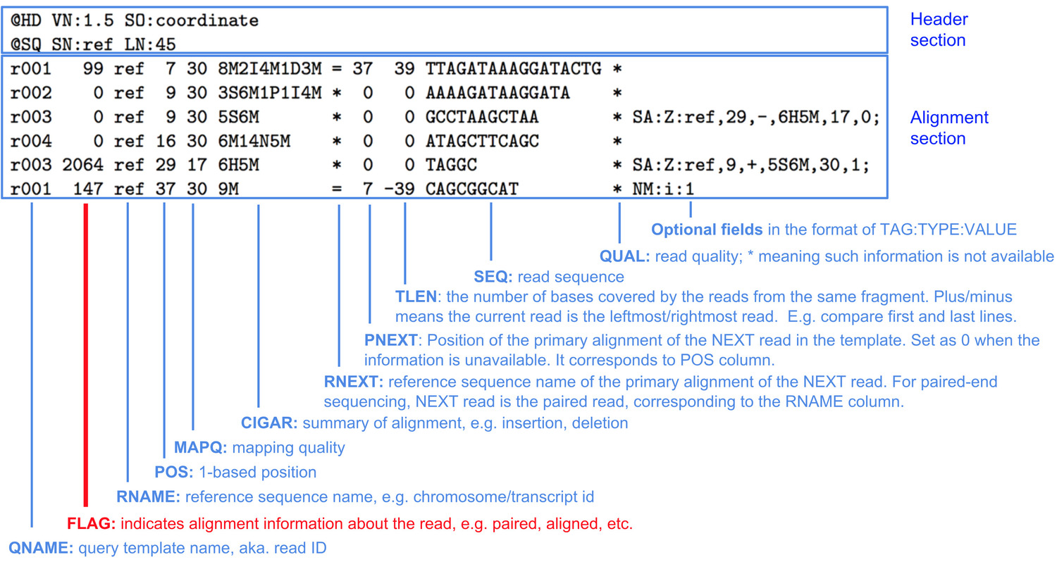 -
- - Header lines start with
@ - Alignment lines include:
- Read name
- Flag
- Reference name
- Position
- Mapping quality
- CIGAR string
- Mate information
- Sequence
- Quality
- Used In: Intermediate results; inspection/debugging of alignments.
3. BAM - Binary Alignment/Map
- Description: Binary, compressed version of SAM.
- Type: Binary
- Benefits:
- Smaller file size
- Faster for analysis and processing
- Used In: Standard format for storing aligned NGS data.
4. CRAM - Compressed Reference-based Format
- Description: Highly compressed alternative to BAM.
- Type: Binary (uses reference-based compression)
- Benefits:
- More storage-efficient than BAM
- Requires access to the reference genome for decompression
- Used In: Large-scale sequencing projects; long-term storage.
5. VCF - Variant Call Format
- Description: Stores genetic variation (SNPs, indels).
- Type: Text-based
- Structure:
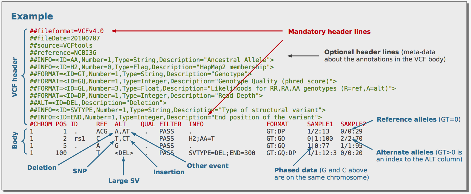
- Fields:
- Chromosome
- Position
- Reference/alternate alleles
- Quality metrics
- Genotype information
- Used In: Output of variant callers (e.g., GATK, FreeBayes).
6. BCF - Binary Call Format
- Description: Binary version of VCF.
- Type: Binary
- Benefits:
- Compact
- Faster for computational tasks
- Used In: Efficient analysis and storage of variant data.
Summary Table
| Format | Type | Purpose | Input/Output for |
|---|---|---|---|
| FASTQ | Text | Raw sequencing reads | Aligners |
| SAM | Text | Aligned reads (human-readable) | Alignment tools |
| BAM | Binary | Compressed aligned reads | Analysis tools |
| CRAM | Binary | Reference-compressed alignments | Archival storage |
| VCF | Text | Genetic variants | Variant callers |
| BCF | Binary | Compressed variant format | Genomic analysis |
Further Reading
Types of Variants in Genomics
Genomic variants refer to differences in the DNA sequence between individuals of a species. Variants can be classified into different categories based on their size, type, and impact on genes and proteins. These DNA changments may be in singleton on in a differences set.

1. Single Nucleotide Variants (SNVs)
SNVs are the most common type of variant and involve a change of a single nucleotide (A, T, C, or G) in the DNA sequence.
- Types:
- Synonymous SNVs: Change the DNA sequence but do not affect the amino acid sequence of the protein.
- Non-synonymous SNVs: Change the DNA sequence and result in an altered amino acid in the protein. These can be:
- Missense: A single amino acid change.
- Nonsense: Results in a premature stop codon, potentially truncating the protein.

2. Insertions and Deletions (Indels)
Indels involve the insertion or deletion of small DNA sequences.
- Insertion: Addition of one or more nucleotides into the DNA sequence.
- Deletion: Removal of one or more nucleotides from the sequence.
- Frameshift: If the number of inserted or deleted nucleotides is not divisible by three, it causes a shift in the reading frame, often leading to a completely different and usually non-functional protein.
3. Structural Variants (SVs)
Structural variants refer to larger changes in the genome, typically affecting more than 50 base pairs. These can involve duplications, deletions, inversions, or translocations of large segments of DNA.
- Types:
- Copy Number Variations (CNVs): Large regions of the genome are duplicated or deleted.
- Inversions: A segment of the chromosome is reversed.
- Translocations: A segment of one chromosome is transferred to another.
4. Tandem Repeats
These are short sequences of DNA that are repeated multiple times in a row.
- Types:
- Short Tandem Repeats (STRs): Typically 2-6 base pairs in length.
- Variable Number Tandem Repeats (VNTRs): Larger repetitive regions.
5. Copy Number Variations (CNVs)
CNVs involve changes in the number of copies of a particular region of the genome. These can be large deletions or duplications and can affect gene dosage, potentially leading to disease.

6. Mobile Element Insertions
Mobile elements (like transposons) can insert themselves into different locations within the genome. These insertions can disrupt normal gene function or regulation.
- Types:
- LINEs: Long interspersed nuclear elements.
- SINEs: Short interspersed nuclear elements.
7. Mitochondrial Variants
Mitochondrial variants occur in the mitochondrial DNA and can affect cellular energy production.
Theoretical Background on Variant Calling
There appear to be no benchmarks for translating WES/WGS into clinical knowledge. This is because different disorders require multiple approaches to basic genomic variant analysis as well as supplemental analyses such as disease-specific interpretation and variant prioritization.Most labs employ workflows that involve several steps that gradually filter and prioritize variants for phenotype cross-correlation to maximize analysis efficiency. The remaining variants are prioritized based on additional characteristics, such as the variant's functional impact [Hedge et al., 2017]. Several bioinformatics tools have advanced in their ability to prioritize candidate disease genes from disease gene loci.
The NGS bioinformatics pipeline describes the set of bioinformatics algorithms used to process NGS data. It is typically a series of transformations that instruct and process massive sequencing data and their associated metadata using multiple software components, databases, and operating environments (hardware and operating systems). Specifying a human reference genome, acknowledging the limitations of predicting copy number and structural variation, establishing algorithms for characterizing genetic variants, evaluating publicly accessible annotation resources, and developing filtering metrics for disease-causing variants are all steps in developing a bioinformatics pipeline (SoRelle et al., 2020].
A comprehensive pipeline that can be applied for WES/WGS data analysis consists of the following steps :
-
Preprocessing of Sequencing Data
- Quality Control (QC) :
Assess the quality of raw sequencing reads to identify and address issues such as low-quality reads, adapter contamination, and sequencing errors. Tools like FastQC are commonly used.
- Trimming and Filtering :
Remove low-quality bases and adapter sequences from reads using tools such as Trimmomatic or Cutadapt.
- Read Alignment :
Align the cleaned reads to a reference genome using aligners like BWA (Burrows-Wheeler Aligner), Bowtie2, or STAR. The result is a file in BAM format, which contains the mapped reads.
- Quality Control (QC) :
-
Post-Alignment Processing
- Sorting :
Organize the aligned reads in the BAM file by their position on the reference genome. This step is typically performed using tools like SAMtools or Picard.
- Marking Duplicates :
Identify and mark duplicate reads that arise from PCR amplification during library preparation, which can lead to biases in variant calling. Tools like Picard’s MarkDuplicates are used.
- Base Quality Score Recalibration (BQSR):
Adjust the base quality scores of reads to correct systematic errors using tools like GATK (Genome Analysis Toolkit).
- Sorting :
-
Variant Calling
- Call Variants :
Detect variants (SNPs and indels) from the processed BAM file. Popular variant callers include GATK HaplotypeCaller, SAMtools, FreeBayes, and Varscan. This step results in a Variant Call Format (VCF) file containing the detected variants.
- Variant Filtering :
Apply filters to the called variants to remove false positives and retain high-confidence variants. Filtering criteria may include read depth, variant allele frequency, and quality metrics. Tools like GATK’s VariantFiltration can be used.
- Call Variants :
-
Variant Annotation and Interpretation
- Annotate Variants :
Enrich the VCF file with functional information about the variants, such as their impact on genes, potential pathogenicity, and clinical relevance. Tools like SnpEff, VEP (Variant Effect Predictor), and ANNOVAR are commonly used for this purpose.
- Interpret Variants :
Evaluate the biological significance of the variants in the context of the disease or phenotype being studied. This involves correlating variants with known disease associations, assessing their functional impact, and integrating other data such as family history or phenotypic information.
- Annotate Variants :
-
Validation and Reporting
- Validate Variants :
Confirm the presence of variants using additional techniques such as Sanger sequencing, especially for critical findings or those with high clinical relevance.
- Generate Reports :
Create comprehensive reports detailing the identified variants, their potential impact, and recommendations based on the analysis. This often involves summarizing findings in a way that is understandable and actionable for clinical or research purposes.
- Validate Variants :
Due to the automated nature of a typical clinical bioinformatics pipeline, adequate quality control (QC) is necessary to ensure that the data collected is reliable, accurate, reproducible, and identifiable. The computing resources required to sequence, process, store, and interpret massive amounts of data are determined by the tools and pipelines used to evaluate such data. Each diagnostic laboratory performing WES and WGS has its own analytical pipeline, demonstrating the size and scope of clinical tools available. These pipelines frequently employ open-source, proprietary, and commercial software. The bottleneck in WGS/WES is data management and computational analysis of raw data, not sequencing itself. Each phase of the analysis workflow must be considered carefully in order to produce meaningful results. This requires the careful selection of tools for these analyses. Most of these tools have the limitation of focusing on a single element of the entire process rather than delivering an automated pipeline that can guide the researcher from start to finish. While sequencing technology and software are essential, so are the internal parameters used by each algorithm, especially the filtering options used by variant callers, which have been shown to affect overall variant call quality.
To the greatest extent possible, laboratories analyze their data using either in-house developed or commercially available software and pipelines. While these pipelines vary by laboratory, a reasonable first approach is to filter out common variants using population databases. Each phase of the data analysis pipeline, from initial raw data processing to downstream variant filtering, plays a crucial role in the final results. Poorly managed data or inappropriate tool usage can lead to erroneous interpretations or missed variants.
GATK pipeline
What is GATK?
The Genome Analysis Toolkit (GATK) is a software package developed by the Broad Institute specifically for the analysis of high-throughput sequencing data. It is designed to facilitate the discovery and genotyping of variants in genomic sequences, such as single nucleotide polymorphisms (SNPs) and insertions/deletions (indels).

Key Features of GATK
-
Robust Data Processing: The toolkit incorporates a series of best practices for data preprocessing, including alignment, duplicate marking, and quality score recalibration, ensuring high-quality input for variant calling.
-
Variant Discovery: GATK provides tools to identify genetic variants from raw sequencing data, enabling researchers to uncover differences in genomes.
-
Genotyping: After variants are called, GATK can also genotype these variants across multiple samples, providing insights into population genetics and disease association studies.
-
Flexible Workflow: GATK supports a wide range of workflows, from small-scale studies to large population genomics projects, and is compatible with various input formats, including BAM and VCF.
-
Comprehensive Documentation: GATK is accompanied by extensive documentation and tutorials, making it accessible to both novice and experienced researchers.
Why Use GATK?
- High Accuracy: GATK employs advanced statistical methods that enhance the accuracy of variant calling and reduce false positives.
- Community Support: As one of the most widely used tools in genomics, GATK has a large user community and frequent updates based on user feedback and advancements in the field.
- Integration with Other Tools: GATK can be easily integrated with other bioinformatics tools for downstream analysis, such as annotation and visualization.
Applications
GATK is used in various fields, including:
- Medical Genomics: Identifying genetic variants associated with diseases.
- Population Genetics: Studying genetic diversity and evolutionary patterns.
- Cancer Genomics: Detecting somatic mutations in tumor samples.
Theoretical Foundations of the GATK Pipeline
1. Data Preprocessing
Alignment
Alignment is the process of mapping sequencing reads to a reference genome. Accurate alignment is crucial, as it affects all subsequent analyses. Tools like BWA (Burrows-Wheeler Aligner) or Bowtie2 are commonly used for this step. The goal is to identify where each read originates from in the reference genome, accounting for potential sequencing errors and biological variations.
Marking Duplicates
During PCR amplification, some DNA fragments may be copied multiple times, resulting in duplicate reads. Marking these duplicates is essential to avoid overestimating variant frequencies. GATK's MarkDuplicates tool identifies and flags these duplicates based on their alignment coordinates.
Base Quality Score Recalibration (BQSR)
Quality scores provided by sequencing platforms may not accurately reflect the true error rates. BQSR adjusts these scores using machine learning models that consider covariates such as the context of the base and the read position. This recalibration enhances the reliability of subsequent variant calling.
2. Variant Calling
HaplotypeCaller
The HaplotypeCaller uses a haplotype-based approach to variant calling. Instead of calling variants for each individual read, it considers the entire local context of the reads. This method increases sensitivity and specificity, particularly in regions of the genome with complex variations. The output is typically a GVCF (Genome Variant Call Format) file, which provides information on both variants and non-variant regions.
GenotypeGVCFs
This step combines multiple GVCFs from different samples into a single VCF file. By using joint genotyping, the tool can leverage information from all samples, improving the accuracy of variant calls and allowing for better detection of rare variants.
3. Variant Filtering
Filtering is critical to eliminate false positive variant calls. GATK provides two main approaches:
- Hard Filters: Set specific thresholds for various quality metrics, such as depth of coverage, quality scores, and more.
- Variant Quality Score Recalibration (VQSR): A more sophisticated approach that uses machine learning to model the quality of variants based on known polymorphisms and various metrics.
4. Annotation
Annotation adds biological context to the variants. Tools like ANNOVAR and VEP can be integrated into the pipeline to provide information on the functional impact of variants, such as whether they affect coding sequences, regulatory regions, or are associated with known diseases.
5. Visualization
Visualization tools like IGV (Integrative Genomics Viewer) allow researchers to manually inspect variant calls in the context of the aligned reads. This step is crucial for validating variant calls and understanding the biological implications of identified variants.
Example Workflow
Step 1: Align reads
bwa mem reference.fasta reads.fastq > aligned.sam
Step 2: Convert SAM to BAM, sort, and mark duplicates
samtools view -Sb aligned.sam | samtools sort -o sorted.bam gatk MarkDuplicates -I sorted.bam -O dedup.bam -M metrics.txt
Step 3: Base Quality Score Recalibration
gatk BaseRecalibrator -I dedup.bam -R reference.fasta --known-sites known_sites.vcf -O recal_data.table gatk ApplyBQSR -I dedup.bam -R reference.fasta --bqsr-recal-file recal_data.table -O recal.bam
Step 4: Variant Calling
gatk HaplotypeCaller -R reference.fasta -I recal.bam -O raw_variants.g.vcf -ERC GVCF
Step 5: Genotype GVCFs
gatk GenotypeGVCFs -R reference.fasta -V raw_variants.g.vcf -O final_variants.vcf
Step 6: Filter variants
gatk VariantFiltration -V final_variants.vcf -O filtered_variants.vcf --filter-expression "QUAL < 30.0" --filter-name "LowQual"
Resources
- Ressource 1: GATK official documentation.
Nf-core Pipelines for Variant Calling
Introduction
Nf-core is a collaborative initiative to provide a curated set of high-quality Nextflow pipelines. It is designed for reproducible and portable workflows that cater to a wide range of bioinformatics applications. In the context of variant calling, nf-core offers robust pipelines that are extensively tested, easy to use, and customizable. Variant calling is a critical step in genomic analysis, identifying variations such as SNPs (single nucleotide polymorphisms) and indels (insertions and deletions) in DNA or RNA sequences.
Key Features of nf-core Pipelines for Variant Calling
- Standardization: Pipelines adhere to best-practice guidelines and community standards.
- Portability: Compatibility with multiple environments (local systems, HPC, cloud).
- Reproducibility: Version-controlled workflows and containers ensure consistent results.
- Customization: Configurable parameters to adapt workflows to specific datasets and research questions.
Commonly Used nf-core Pipelines for Variant Calling
1. nf-core/sarek
- Purpose: Comprehensive pipeline for germline and somatic variant calling.
- Supported Analysis:
- Preprocessing: Alignment, recalibration, and quality control.
- Variant calling with tools like GATK, Mutect2, Strelka, FreeBayes, etc.
- Annotation and filtering of variants.
- Highlights:
- Multimodal: Supports both WGS and WES data.
- Scalability: Handles both small-scale and large-scale datasets.
2. nf-core/somaticseq
- Purpose: Focused on somatic mutation detection.
- Key Features:
- Combines multiple variant callers for enhanced accuracy.
- Utilizes machine learning to improve sensitivity and specificity.
3. nf-core/rna-seq
- Purpose: Primarily for RNA-seq data analysis, but supports variant calling on transcriptome data.
- Highlights:
- High-quality alignment with STAR or HISAT2.
- Variant calling on RNA-seq using tools like GATK HaplotypeCaller.
Getting Started
-
Installation:
- Install Nextflow:
curl -s https://get.nextflow.io | bash - Pull the desired pipeline:
nextflow pull nf-core/<pipeline_name>
- Install Nextflow:
-
Execution:
- Run the pipeline with a configuration file or CLI arguments:
nextflow run nf-core/sarek -profile <docker/singularity/conda> --input samplesheet.csv --genome GRCh38
- Run the pipeline with a configuration file or CLI arguments:
-
Configuration:
- Customize the workflow by editing
paramsor providing a custom configuration file.
- Customize the workflow by editing
Best Practices
- Use proper genome references and annotations (e.g., GRCh38, hg19).
- Follow nf-core documentation to ensure proper usage of profiles (
docker,singularity, etc.). - Use MultiQC for summarizing QC metrics.
Conclusion
Nf-core pipelines streamline the complex workflows of variant calling, ensuring reproducibility, scalability, and reliability. Whether analyzing germline variants, somatic mutations, or RNA-seq derived variations, nf-core offers tailored solutions for every need.
- Ressource 1: nf-core Website .
- Ressource 2: Nextflow Documentation .
Tools
Choosing the right tools for NGS (Next-Generation Sequencing) analysis involves several key considerations:
-
Define Your Goals: Clearly outline your objectives (e.g., variant calling, transcriptome analysis, metagenomics) to narrow down suitable tools.
-
Data Type: Consider the type of NGS data you have (e.g., DNA-seq, RNA-seq, ChIP-seq) as tools are often optimized for specific data types.
-
Scalability: Ensure the tools can handle your data size. Some tools are better suited for large datasets or high-throughput analyses.
-
Accuracy and Reliability: Look for tools with proven performance and community support. Check published studies or benchmarks for validation.
-
User-Friendly Interface: If you’re not very experienced, opt for tools with graphical user interfaces (GUIs) or comprehensive documentation.
-
Integration with Other Tools: Consider tools that can integrate well with existing pipelines or workflows, particularly in a bioinformatics framework.
-
Community and Support: Active user communities and available support can be invaluable for troubleshooting and learning.
-
Cost and Licensing: Assess whether the tools are open-source or require licensing fees, as budget constraints can influence your choice.
-
Computational Requirements: Evaluate the hardware requirements and whether you have the necessary computational resources available.
-
Reproducibility: Opt for tools that support reproducible research practices, allowing for easier sharing and validation of results.
single nucleotide variant calling
| Name | Published | Control Needed | Indel Detection | Contamination Correction | Ref |
|---|---|---|---|---|---|
| Varscan2 | 2012 | + | + | − | 1 |
| MuTect2 * | 2013 | + | − | + | 2 |
| FreeBayes | 2012 | − | + | − | 3 |
| Strelka * | 2012 | + | + | − | 4 |
| Platypus * | 2014 | − | + | − | 5 |
| SomaticSniper * | 2012 | + | − | − | 6 |
| LoFreq * | 2012 | − | + | + | 7 |
| VarDict * | 2016 | − | + | − | 8 |
| JointSNVMix * | 2012 | + | − | − | 9 |
| MutationSeq * | 2012 | + | − | − | 10 |
| EBCall * | 2013 | + | + | − | 11 |
| MuSE * | 2016 | + | − | + | 12 |
| RADIA | 2014 | + | − | + | 13 |
| Virmid | 2013 | + | − | + | 14 |
| deepSNV * | 2014 | + | − | − | 15 |
| Shimmer * | 2013 | + | − | + | 16 |
| qSNP * | 2013 | + | − | + | 17 |
| BAYSIC | 2014 | + | − | − | 18 |
| SomaticSeq * | 2015 | + | + | − | 19 |
| CaVEMan * | 2016 | + | − | + | 20 |
| SNooPer * | 2016 | − | + | + | 21 |
| SNVSniffer * | 2016 | − | + | − | 22 |
| HapMuC | 2014 | − | + | − | 23 |
| FaSD-somatic | 2014 | − | − | − | 24 |
| LocHap * | 2016 | + | + | + | 25 |
| LoLoPicker * | 2017 | + | − | + | 26 |
Copy Number Variations
| Name | Published | Control Needed | Contamination Correction | GC-Content Correction | REF |
|---|---|---|---|---|---|
| Varscan2 | 2012 | + | − | − | 1 |
| CNVnator | 2011 | + | − | + | 2 |
| CNV-Seq | 2009 | + | − | − | 3 |
| CoNIFER | 2012 | − | + | − | 4 |
| Control-FREEC | 2012 | − | + | + | 5 |
| ExomeCNV | 2011 | + | + | − | 6 |
| XHMM | 2012 | − | + | + | 7 |
| ExomeDepth | 2012 | + | − | + | 8 |
| cn.MOPS | 2012 | − | + | + | 9 |
| Cnvkit | 2016 | + | + | + | 10 |
| CONTRA | 2012 | − | − | + | 12 |
| Sequenza | 2015 | + | − | + | 13 |
| EXCAVATOR | 2013 | + | + | + | 14 |
| CODEX | 2015 | − | + | + | 16 |
| ADTEx | 2014 | + | − | + | 17 |
| Seqgene | 2011 | + | − | − | 18 |
| FishingCNV | 2013 | − | − | − | 19 |
| HMZDelFinder | 2017 | − | − | − | 20 |
| ExoCNVTest | 2012 | + | − | − | 21 |
| CLAMMS | 2016 | − | − | + | 22 |
| falcon | 2015 | + | + | − | 23 |
| saasCNV | 2015 | + | + | − | 24 |
| WISExome | 2017 | − | − | − | 25 |
| GATK |
Structural Variations
| Name | Description | REF |
|---|---|---|
| Manta | Manta is a structural variant caller developed by Illumina. It detects various types of SVs, including deletions, duplications, inversions, and translocations. Works with whole-genome and exome sequencing data. | 1 |
| Delly | Delly is a versatile SV detection tool that can identify deletions, duplications, inversions, translocations, and more. It works with various sequencing data types, including exome data. | 2 |
| Lumpy | Lumpy focuses on identifying interchromosomal translocations and intrachromosomal rearrangements. It can be adapted for use with exome data. | 3 |
| BreakDancer | Pindel detects breakpoints of large deletions, medium-sized insertions, inversions, tandem duplications, and other structural variants. Suitable for both whole-genome and exome data. | 4 |
| GRIDSS | GRIDSS is a versatile SV caller that can detect complex structural variants by combining multiple evidence types. Suitable for various sequencing data types, including exome data. | 5 |
| CNVkit | CNVkit is primarily for copy number variation detection but can also identify large-scale structural variations from exome data by analyzing read depth. | 6 |
| TIDDIT | TIDDIT is designed for identifying tandem duplications and can be used with exome sequencing data to detect this specific type of structural variation. | 7 |
Splicing Site Detection
| Name | Description | REF |
|---|---|---|
| SpliceAI | SpliceAI is a deep learning-based tool that predicts the effect of variants on splicing, providing information about splice site alterations. | 1 |
| Human Splicing Finder (HSF) | HSF is a web-based tool that predicts the potential impact of variants on splicing, analyzing consensus splice site sequences for potential disruptions. | 2 |
| MMSplice | MMSplice is a machine learning-based tool that predicts the impact of variants on alternative splicing events, providing a score for splicing disruption likelihood. | 3 |
| SplicePort | SplicePort is a web-based tool that predicts the potential impact of variants on splice site creation or disruption, considering both donor and acceptor splice sites. | 4 |
Annotation
| Name | Description | REF |
|---|---|---|
| Annovar | ANNOVAR is a versatile tool for annotating genetic variants, providing information on variant function, population allele frequencies, and predicted functional consequences. | 1 |
| SnpEff | SnpEff annotates genetic variants, categorizing them based on functional impact and providing annotations on genes and transcripts. | 2 |
| dbNSFP | The Database for Non-Synonymous SNPs' Functional Predictions (dbNSFP) provides functional predictions for non-synonymous variants in exomes, including predictions from multiple tools. | 3 |
| Exomiser | Exomiser prioritizes and annotates variants in exome data for rare disease research, integrating variant data with various databases and gene-phenotype information. | 4 |
| VCFanno | VCFanno is a flexible tool for annotating VCF files, allowing customization of annotation sources and rules. | 5 |
| VEP | VEP is a powerful tool from Ensembl for annotating genetic variants, offering insights into functional effects, gene impacts, regulatory regions, and population allele frequencies. | 6 |
| VariantDB | VariantDB is a platform for variant annotation and interpretation, providing various annotation sources and custom annotation tracks. | 7 |
| GnomAD | The Genome Aggregation Database (gnomAD) offers access to allele frequencies of genetic variants in large populations, useful for annotating exome variants. | 8 |
| ClinVar | ClinVar is a database of clinically relevant variants, providing annotations related to clinical significance and associations with diseases. | 9 |
| OMIM | OMIM is a comprehensive database of genetic disorders and associated genes, useful for annotating exome variants with disease-related information. | 10 |
- Ressource 1: Comprehensive Outline of Whole Exome Sequencing Data Analysis Tools Available in Clinical Oncology .
- Ressource 2: A Survey of Computational Tools to Analyze and Interpret Whole Exome Sequencing Data .
- Ressource 3: Review on the Computational Genome Annotation of Sequences Obtained by Next-Generation Sequencing.
Statistical Models in Identifying Variants from NGS Data
Next-Generation Sequencing (NGS) technology generates vast amounts of genomic data, enabling unprecedented insights into genetic variation. However, this data is not error-free, and distinguishing true genetic variants from artifacts is a critical step. Statistical models serve as the foundation for this process, providing robust methods to interpret sequencing reads accurately.
Why Statistical Models Matter
NGS data comes with inherent challenges such as sequencing errors, alignment issues, and variability in read depth. Statistical models are tailored to account for these complexities by incorporating probabilities, data distributions, and machine learning techniques to enhance variant calling precision.
Below, we outline some of the most widely used statistical models in the analysis of NGS data.
1. Bayesian Models: Precision Through Probabilities
Bayesian inference is a cornerstone of variant calling, where prior knowledge and observed data converge to estimate the likelihood of a variant.
- Applications: Bayesian models are integral to tools like GATK HaplotypeCaller, which calls SNPs and indels.
- Strengths: These models can incorporate diverse data types, such as base quality scores, allele frequency, and mapping quality.
- Real-world Use: For example, Bayesian approaches help resolve low-frequency variants in mixed samples.
2. Maximum Likelihood Estimation (MLE): Maximizing Fit
MLE seeks to identify model parameters that maximize the likelihood of observing the given sequencing data.
- Applications: Found in popular tools such as Samtools and FreeBayes.
- Key Insight: By balancing the number of reads supporting a reference or alternate allele, MLE ensures robust variant detection.
3. Hidden Markov Models (HMM): Uncovering the Hidden
HMMs are statistical models that excel in analyzing sequential data, making them ideal for identifying genomic regions with variations.
- Applications: Utilized in tools like Platypus for phasing and variant detection.
- Advantages: By accounting for dependencies between adjacent positions, HMMs can identify variants in complex regions.
4. Poisson and Negative Binomial Models: Modeling Read Distributions
The distribution of sequencing reads across the genome can reveal structural variations and copy number changes.
- Applications: Commonly used in RNA-Seq and CNV detection workflows.
- Technical Edge: While Poisson assumes uniformity, the Negative Binomial model accounts for variability, making it more suited to overdispersed data.
5. Machine Learning Models: The Future of Variant Calling
Machine learning is revolutionizing genomics by leveraging complex patterns in sequencing data.
- Tools: State-of-the-art tools like DeepVariant and Mutect2 employ neural networks and other ML techniques.
- Advantages: Unlike traditional methods, ML adapts to diverse data landscapes, offering unparalleled accuracy in variant calling.
6. Logistic Regression: A Simpler Yet Effective Approach
Logistic regression remains a workhorse for filtering variants, especially in somatic mutation detection.
- How It Works: Features like allele frequency, strand bias, and base quality are combined into a probability model.
- Applications: Logistic regression often complements other statistical methods to reduce false positives.
7. Generalized Linear Models (GLMs): Flexibility in Variant Detection
GLMs extend linear regression to handle non-normal data, making them ideal for complex genomic analyses.
- Applications: Used in models that detect tumor-specific variants or account for allele-specific expression.
- Strengths: Their flexibility ensures compatibility with various data types and distributions.
8. Multivariate Models: Joint Variant Calling
For cohort studies, multivariate models allow simultaneous analysis of multiple samples.
- Applications: Joint calling in tools like GATK's GenotypeGVCFs improves accuracy by leveraging population-level data.
- Impact: These models can detect rare variants and improve overall sensitivity.
9. Markov Chain Monte Carlo (MCMC): Handling Uncertainty
MCMC methods sample from probability distributions to estimate variant likelihoods in uncertain scenarios.
- Applications: Ideal for low-frequency variant detection, especially in tumor sequencing.
- Advantages: These methods provide a robust way to model uncertainty in variant calls.
Challenges and Opportunities
While statistical models have advanced variant calling significantly, challenges remain. Regions of low complexity, repetitive sequences, and low-coverage areas continue to test even the best algorithms. However, innovations like machine learning and hybrid approaches are paving the way for more accurate and comprehensive genomic analyses.
Statistical models are the backbone of NGS data interpretation. By integrating biological knowledge with cutting-edge algorithms, these models enable researchers to unlock the secrets of the genome with precision and confidence.
Challenges and pitfalls in detecting variants.
Variant detection is a critical step in genomic analysis, with applications ranging from disease research to personalized medicine. However, the process is fraught with challenges and potential pitfalls that can impact the accuracy, reproducibility, and interpretability of results. This document highlights the common issues and offers insights into their mitigation.
Challenges in Variant Detection
1. Sequencing Errors
- Description: Next-generation sequencing (NGS) technologies can introduce errors such as base miscalls, indels, or low-quality reads.
- Impact: False-positive variants may arise from these errors.
- Mitigation:
- Use high-quality sequencing platforms with low error rates.
- Perform base quality score recalibration and error correction.
2. Low Coverage Regions
- Description: Insufficient read depth in certain genomic regions reduces the confidence in variant calls.
- Impact: Missed true variants or increased false negatives.
- Mitigation:
- Increase sequencing depth.
- Use imputation or specialized tools for low-coverage regions.
3. Alignment Errors
- Description: Poor read alignment, particularly in repetitive or GC-rich regions, can lead to incorrect variant calls.
- Impact: False positives or incorrect variant annotation.
- Mitigation:
- Use advanced aligners like BWA or STAR.
- Apply post-alignment refinement, such as realignment around indels.
4. Complex Genomic Regions
- Description: Highly repetitive or structurally complex regions are challenging for variant detection algorithms.
- Impact: Variants in these regions may be undetected or misclassified.
- Mitigation:
- Employ specialized tools for structural variant detection (e.g., Manta, Delly).
- Use long-read sequencing technologies for better resolution.
5. Reference Genome Bias
- Description: Variants may be misclassified or overlooked if they deviate significantly from the reference genome.
- Impact: Underrepresentation of certain populations or haplotypes.
- Mitigation:
- Use updated and diverse reference genomes.
- Integrate pan-genome approaches to reduce bias.
6. Variant Calling and Filtering
- Description: Different variant callers use varied algorithms and may produce inconsistent results. Poor filtering thresholds can lead to incorrect conclusions.
- Impact: False positives, false negatives, or both.
- Mitigation:
- Compare results from multiple variant callers.
- Apply appropriate quality filtering and recalibration techniques.
7. Annotation Challenges
- Description: Variant annotation tools rely on existing databases that may be incomplete or biased.
- Impact: Inaccurate functional or clinical interpretations of variants.
- Mitigation:
- Use multiple annotation tools and up-to-date databases.
- Cross-reference findings with experimental or functional studies.
8. Somatic Variant Detection
- Description: Tumor samples often have subclonal populations, making it hard to detect low-frequency somatic variants.
- Impact: Missed or incorrect somatic mutations.
- Mitigation:
- Use tools like Mutect2 or Strelka optimized for somatic variant calling.
- Sequence matched normal-tumor pairs to improve accuracy.
Pitfalls in Variant Detection
1. Overconfidence in Variant Callers
- Issue: Over-reliance on a single tool may lead to biased results.
- Solution: Validate findings with multiple tools and experimental methods.
2. Ignoring Batch Effects
- Issue: Technical differences between sequencing runs can introduce batch effects.
- Solution: Standardize protocols and perform batch effect normalization.
3. Neglecting Population Diversity
- Issue: Focusing on a single population reference may overlook variants unique to other groups.
- Solution: Use diverse reference panels like 1KGP or gnomAD.
4. Insufficient Validation
- Issue: Lack of experimental validation may lead to erroneous conclusions.
- Solution: Validate key findings using orthogonal methods like Sanger sequencing or qPCR.
5. Over-Filtering
- Issue: Stringent quality thresholds may remove true positive variants.
- Solution: Balance sensitivity and specificity in filtering criteria.
Conclusion
Detecting variants is a complex process that requires careful attention to sequencing quality, computational tools, and biological interpretation. Awareness of challenges and pitfalls, combined with robust validation strategies, is essential to ensure reliable results in genomic analysis.
By addressing these issues, researchers can improve the accuracy and reliability of their variant detection workflows and contribute to advancements in genomics.
Role of Next-Generation Sequencing (NGS) in Studying Population Genetics and Evolutionary Genomics
Next-Generation Sequencing (NGS) has revolutionized the fields of population genetics and evolutionary genomics by providing unprecedented access to genomic data at scale. It enables researchers to study genetic variation, evolutionary processes, and species diversity with high precision. This document outlines the key contributions of NGS in these fields.
Key Applications of NGS in Population Genetics
1. Characterizing Genetic Variation
- Description: NGS enables genome-wide identification of single nucleotide polymorphisms (SNPs), insertions/deletions (indels), and structural variants.
- Impact:
- Facilitates population-level studies of genetic diversity.
- Identifies loci under selection or associated with traits.
2. Genome-Wide Association Studies (GWAS)
- Description: By sequencing multiple individuals, NGS identifies genetic markers associated with traits or diseases.
- Impact:
- Advances our understanding of the genetic basis of complex traits.
- Provides insights into the heritability of traits in populations.
3. Estimating Population Structure
- Description: NGS data supports fine-scale analysis of population structure and admixture using tools like STRUCTURE and ADMIXTURE.
- Impact:
- Uncovers historical migration patterns and population connectivity.
- Detects signatures of gene flow and hybridization events.
4. Demographic History Inference
- Description: NGS data informs models of population size changes, bottlenecks, and expansions.
- Impact:
- Helps reconstruct ancestral population dynamics.
- Enhances our understanding of evolutionary pressures.
Key Applications of NGS in Evolutionary Genomics
1. Studying Speciation and Divergence
- Description: NGS enables comparative genomic analysis between species or populations.
- Impact:
- Identifies regions of the genome involved in reproductive isolation.
- Explores divergence times and evolutionary relationships.
2. Adaptive Evolution Studies
- Description: Detects genomic regions under natural selection using methods like selective sweeps or FST outliers.
- Impact:
- Reveals adaptations to environmental changes or ecological niches.
- Links genomic changes to phenotypic evolution.
3. Paleogenomics
- Description: NGS retrieves DNA from ancient samples to study extinct species and ancestral populations.
- Impact:
- Reconstructs evolutionary relationships and timelines.
- Investigates the genetic basis of extinction or adaptation.
4. Molecular Evolution
- Description: Analyzes patterns of nucleotide and amino acid changes across genomes.
- Impact:
- Measures rates of evolution (e.g., dN/dS).
- Identifies functional constraints and evolutionary conservation.
Advantages of NGS in Population Genetics and Evolutionary Genomics
-
High Throughput
- Generates vast amounts of data, enabling genome-wide studies.
-
Cost-Effectiveness
- Drastically reduces the cost per base compared to Sanger sequencing.
-
Resolution
- Provides single-base resolution for studying genetic variation.
-
Flexibility
- Suitable for diverse applications, from whole-genome sequencing to targeted resequencing.
-
Accessibility
- Makes genomic studies feasible for non-model organisms.
Challenges and Considerations
- Data Analysis
- Requires advanced computational tools and expertise.
- Data Quality
- Sequencing errors and low coverage can impact results.
- Ethical Concerns
- Population genetic studies must address privacy and consent issues.
- Bias in Sampling
- Unequal representation of populations can skew results.
Conclusion
NGS has transformed population genetics and evolutionary genomics by providing comprehensive insights into genetic variation, evolutionary history, and adaptive processes. As sequencing technologies continue to evolve, they will further enhance our ability to explore the complexity of genomes and their roles in shaping the diversity of life.
References
- Ellegren, H. (2014). Genome sequencing and population genomics. Current Opinion in Genetics & Development.
- Nielsen, R. et al. (2017). Recent advances in population genomics. Nature Reviews Genetics.
Overview of variant annotation and its importance.
Variant annotation is the process of adding meaningful biological information to genetic variants identified through sequencing data. It involves interpreting raw variant calls (e.g., SNPs, indels) by associating them with potential biological consequences, including their effect on gene function, disease association, and population frequencies.
Steps in Variant Annotation
- Gene Annotation: Identifying the gene or genes affected by the variant, and determining whether the variant is in a coding or non-coding region.
- Effect Prediction: Predicting how the variant alters the gene or protein function (e.g., synonymous, missense, nonsense, frameshift).
- Clinical Significance: Determining whether the variant is benign, pathogenic, or of uncertain significance by comparing it against databases like ClinVar or OMIM.
- Population Frequency: Comparing the variant to large-scale population databases (e.g., gnomAD, 1000 Genomes) to determine if it is rare or common in certain populations.
- Functional Impact: Assessing the impact of the variant on protein function or regulation, using tools like SIFT, PolyPhen-2, and CADD.
- Disease Association: Identifying whether the variant is associated with known diseases or phenotypes.
Importance of Variant Annotation
- Disease Diagnosis: Helps clinicians identify pathogenic variants linked to genetic disorders.
- Therapeutic Decisions: Plays a role in precision medicine by identifying actionable variants for targeted therapies.
- Population Genetics: Assists in understanding the distribution of genetic variations across different populations, contributing to evolutionary studies.
- Functional Genomics: Helps researchers discover how variants affect gene expression, protein function, and biological pathways.
- Variant Prioritization: Essential for filtering large sets of variants, focusing on those with clinical relevance or significant functional impact.
Accurate variant annotation is key to translating genomic data into actionable clinical and biological insights.
How Variant Annotation is Done
Variant annotation involves the application of computational tools and databases to systematically interpret genetic variants discovered through next-generation sequencing (NGS). Here’s a more detailed breakdown of how the annotation process is carried out:
1. Variant Identification
Before annotation, the variants (single nucleotide polymorphisms [SNPs], insertions, deletions, structural variants) need to be identified using variant calling pipelines. Tools such as GATK (Genome Analysis Toolkit), FreeBayes, or DeepVariant analyze raw sequencing data (FASTQ files) and generate variant call files (VCF format).
2. Annotation Tools
There are several well-established tools used to annotate variants. These tools incorporate reference genomes, gene annotations, population data, and other functional information. Examples include:
- ANNOVAR: Annotates variants with information from multiple databases (e.g., RefSeq, dbSNP, 1000 Genomes).
- VEP (Variant Effect Predictor): Developed by Ensembl, it predicts the functional effects of genetic variants.
- SnpEff/SnpSift: Focuses on functional impact predictions and has a streamlined pipeline for clinical variant interpretation.
These tools automate the variant annotation process, streamlining the addition of biological meaning.
3. Databases Used in Annotation
Annotation tools rely on diverse data sources, such as:
- Population Databases: Databases like gnomAD, 1000 Genomes, and ExAC provide allele frequencies across global populations. This helps determine if a variant is rare or common.
- Disease Databases: ClinVar, OMIM, HGMD provide curated information on clinically relevant variants associated with diseases.
- Gene Annotations: Databases like Ensembl, UCSC Genome Browser, and RefSeq provide detailed information on gene structure, transcripts, and regulatory elements.
- Functional Prediction Tools: Tools like SIFT, PolyPhen-2, and CADD predict the functional impact of coding variants (e.g., whether a missense mutation is likely to disrupt protein function).
4. Variant Annotation Workflow
The process of annotating variants generally follows these steps:
Step 1: Preprocessing
- Quality Control: Ensure high-quality variant calls (e.g., using filters like depth of coverage, Phred scores, variant quality).
- Format Conversion: Convert the VCF or other formats into a form compatible with the annotation tools (some tools accept only specific formats).
Step 2: Gene Mapping
- Map Variants to Genes: Each variant is assigned to its genomic location. If it’s within a gene, tools like ANNOVAR and VEP map the variant to the appropriate gene, exon, or regulatory region.
- Coding Region Variants: If the variant affects coding sequences, it is annotated with changes to amino acid sequences (missense, nonsense, synonymous).
- Non-Coding Region Variants: Variants in introns, promoters, or UTRs are annotated with their potential impact on gene regulation or splicing.
Step 3: Effect Prediction
- Functional Impact: Functional tools predict the potential consequence of variants:
- SIFT: Predicts whether an amino acid substitution will affect protein function based on evolutionary conservation.
- PolyPhen-2: Assesses the possible impact of amino acid changes on the structure and function of a protein.
- CADD: Scores the deleteriousness of both coding and non-coding variants.
Step 4: Clinical Relevance
- Compare with Known Variants: Annotators check databases like ClinVar for any known associations between a given variant and diseases.
- If a variant matches one in the database, it might be classified as pathogenic, likely pathogenic, benign, or variant of uncertain significance (VUS).
Step 5: Population Frequencies
- Check Population Frequencies: Rare variants, especially those with a frequency below 1% in global databases like gnomAD or 1000 Genomes, are more likely to be associated with diseases. Common variants tend to be benign unless associated with complex traits.
Step 6: Variant Prioritization
- Prioritization Criteria: Based on clinical significance, population rarity, and predicted functional impact, variants are prioritized for further investigation.
- Tier 1: Variants already known to be pathogenic (e.g., in ClinVar).
- Tier 2: Predicted deleterious variants in disease-related genes.
- Tier 3: Rare variants with uncertain significance that may warrant further functional validation.
5. Output of Variant Annotation
The final result is typically a table or report that includes the following key elements for each variant:
- Chromosome and Position: The genomic location.
- Reference and Alternative Alleles: The nucleotide change.
- Gene Name: The gene impacted by the variant.
- Variant Effect: The type of mutation (e.g., synonymous, missense).
- Functional Predictions: Scores from SIFT, PolyPhen-2, CADD, etc.
- Population Frequency: Allele frequencies from databases like gnomAD.
- Disease Association: Any associated disease or trait.
- Clinical Significance: Whether the variant is pathogenic, benign, or VUS.
6. Challenges and Considerations
- VUS (Variant of Uncertain Significance): A large proportion of rare variants have unknown clinical significance, which makes their interpretation challenging.
- Interpretation of Non-Coding Variants: Non-coding variants often lack clear functional annotation, though emerging tools are improving prediction in these regions.
- Data Integration: Combining population, clinical, and functional data into a coherent interpretation requires expert knowledge and sometimes manual curation.
7. Tools for Visualization
Some variant annotation workflows include visual tools that help researchers explore and interpret data. Tools like IGV (Integrative Genomics Viewer) provide a graphical representation of variants in the context of their genomic locations.
Predicting the Impact of Variants on Gene Function (Pathogenicity Scoring)
Understanding how genetic variants impact gene function is essential, especially in fields like clinical genomics, where it helps us determine whether a variant is likely to cause disease. Over time, scientists have developed several computational tools to predict the functional and clinical significance of variants. These tools analyze features such as evolutionary conservation, protein structure, and how common a variant is in the population to estimate its potential impact on gene function and its likelihood of causing disease.
Key Approaches to Predicting Pathogenicity
Pathogenicity scoring tools can generally be grouped into two main types:
- Functional Impact Prediction: These tools try to predict whether a variant will disrupt protein function or gene expression.
- Clinical Pathogenicity Scoring: These tools focus on assessing the chance that a variant is associated with a disease.
Popular Pathogenicity Scoring Algorithms
1. SIFT (Sorting Intolerant From Tolerant)
- What it does: SIFT predicts whether an amino acid change will affect protein function by looking at how much that part of the protein has been conserved across different species.
- How it works: If a particular amino acid is often conserved, a change there might be harmful. SIFT gives scores between 0 and 1. A score ≤0.05 means the change is likely harmful, while scores above 0.05 mean it's probably fine.
2. PolyPhen-2 (Polymorphism Phenotyping v2)
- What it does: PolyPhen-2 predicts whether an amino acid change will impact the structure or function of a protein.
- How it works: It uses information like how conserved the sequence is and how the structure of the protein might change. It categorizes variants as probably damaging, possibly damaging, or benign.
3. CADD (Combined Annotation Dependent Depletion)
- What it does: CADD scores both coding and non-coding variants for their potential deleterious effects.
- How it works: It uses a combination of many features, including conservation and regulatory annotations, to come up with a score. A score above 20 usually indicates a variant in the top 1% of deleterious variants.
4. MutationTaster
- What it does: MutationTaster predicts the disease-causing potential of various types of variants, including amino acid changes and small insertions or deletions.
- How it works: It looks at evolutionary conservation, splicing effects, and other gene-related information to classify a variant as either disease-causing or polymorphism.
5. FATHMM (Functional Analysis through Hidden Markov Models)
- What it does: FATHMM predicts the functional impact of coding and non-coding variants.
- How it works: It uses evolutionary conservation and sequence similarity across species to assess the likelihood of a variant being harmful. The lower the score, the more likely the variant is harmful.
6. REVEL (Rare Exome Variant Ensemble Learner)
- What it does: REVEL focuses on missense variants and uses machine learning to predict their pathogenicity.
- How it works: It combines predictions from other tools (like SIFT, PolyPhen-2, etc.) to come up with a consensus score. Higher scores mean a higher likelihood of pathogenicity.
7. PrimateAI
- What it does: PrimateAI uses deep learning to predict the likelihood that a missense variant will be pathogenic.
- How it works: It compares data from primates and other species to assess evolutionary conservation. Scores range from 0 to 1, with higher scores indicating a greater chance the variant is harmful.
8. DANN (Deleterious Annotation of Genetic Variants using Neural Networks)
- What it does: DANN predicts the pathogenicity of both coding and non-coding variants using deep learning.
- How it works: It analyzes genomic features and annotations and assigns a score between 0 and 1, with higher scores indicating a greater likelihood of being harmful.
9. ClinPred
- What it does: ClinPred predicts the clinical significance of a variant.
- How it works: It integrates features like evolutionary conservation and allele frequencies to estimate whether a variant is pathogenic or benign.
10. Eigen/Eigen-PC
- What it does: Eigen scores the deleteriousness of both coding and non-coding variants using functional genomic data.
- How it works: It applies principal component analysis (PCA) to various genomic features to generate a score, with Eigen-PC refining the scores by incorporating known pathogenic variants.
11. M-CAP (Mendelian Clinically Applicable Pathogenicity)
- What it does: M-CAP improves the classification of rare missense variants, especially in Mendelian diseases.
- How it works: It combines functional prediction scores (like SIFT, PolyPhen-2, CADD) with clinical features to generate a final score.
12. VEST (Variant Effect Scoring Tool)
- What it does: VEST predicts the pathogenicity of non-synonymous variants, particularly in cancer-related genes.
- How it works: It uses machine learning to analyze multiple types of data and produce a score. Higher scores indicate a higher likelihood of pathogenicity.
13. MutPred
- What it does: MutPred predicts how amino acid substitutions affect the molecular function of proteins.
- How it works: It uses machine learning to analyze the molecular changes that might be caused by a variant, giving a probability score indicating the likelihood of pathogenicity.
Using Pathogenicity Scoring in Clinical Contexts
In clinical genomics, these scoring tools are often combined to make more informed predictions. The American College of Medical Genetics and Genomics (ACMG) guidelines suggest integrating multiple lines of evidence when classifying variants. These guidelines help clinicians determine whether a variant is pathogenic, likely pathogenic, benign, or a variant of uncertain significance (VUS), by considering factors like:
- Population data,
- Computational predictions,
- Functional studies,
- Family history, and
- Clinical observations.
Example Workflow for Predicting Pathogenicity:
- Identify variants: Use sequencing data to find variants.
- Run predictions: Apply algorithms like SIFT, PolyPhen-2, REVEL, and CADD to assess each variant.
- Cross-reference with databases: Compare the results with known data from resources like ClinVar and OMIM.
- Expert review: Have experts manually review the data to ensure consistency with clinical findings and the latest research.
Pathogenicity scoring tools provide a starting point for evaluating the potential impact of variants, using a range of data sources like evolutionary conservation and protein function. Since no single tool is perfect, it’s common practice to combine the results from multiple algorithms to make more reliable predictions. In clinical settings, these tools are key for determining whether a genetic variant is likely to be disease-causing, helping clinicians make informed decisions for patients.
These algorithms have revolutionized how we analyze genetic data, especially in the context of diagnosis and personalized medicine..
ACMG Criteria for Clinical Use
The American College of Medical Genetics and Genomics (ACMG) has established a framework for the interpretation of genetic variants in clinical settings. These criteria are critical for standardizing variant classification and ensuring consistent and accurate genetic diagnoses.
Overview of ACMG Guidelines
The ACMG framework classifies variants into five categories based on their pathogenicity:
- Pathogenic (P)
- Likely Pathogenic (LP)
- Uncertain Significance (VUS)
- Likely Benign (LB)
- Benign (B)
The classification process involves evaluating evidence from multiple sources, including population data, computational predictions, functional studies, and clinical observations.
Key Criteria Categories
1. Population Data
- Benign Evidence: Variant frequency significantly higher than expected for a disorder (e.g., >5% in a population database).
- Pathogenic Evidence: Variant absent or extremely rare in population databases (e.g., ExAC, gnomAD).
2. Computational and Predictive Data
- Pathogenic Evidence: Multiple in silico tools predict a deleterious effect on protein function or splicing (e.g., SIFT, PolyPhen).
- Benign Evidence: Predictive tools indicate a lack of impact on protein function.
3. Functional Data
- Pathogenic Evidence: Well-established functional studies demonstrate a deleterious effect.
- Benign Evidence: Studies show no functional impact.
4. Segregation and Co-Segregation
- Pathogenic Evidence: Variant segregates with disease in multiple affected family members.
- Benign Evidence: Lack of segregation in family studies.
5. De Novo Occurrence
- Pathogenic Evidence: Variant arises de novo in an affected individual, with confirmed parentage.
6. Allelic Data
- Pathogenic Evidence: Variant observed in trans with a pathogenic variant in recessive diseases or in cis with another pathogenic variant in dominant diseases.
- Benign Evidence: Co-occurrence with a pathogenic variant in a different gene responsible for the observed phenotype.
7. Clinical Evidence
- Pathogenic Evidence: Variant previously reported in multiple affected individuals or families with consistent phenotypes.
- Benign Evidence: Variant consistently observed in unaffected individuals.
Strength of Evidence
Each criterion is assigned a strength level:
- Very Strong (PVS1): Null variant in a gene where loss-of-function is a known mechanism of disease.
- Strong (PS): E.g., functional evidence or co-segregation.
- Moderate (PM): E.g., moderate population frequency, computational evidence.
- Supporting (PP): E.g., specific phenotypic match.
The evidence is integrated using a structured framework to classify the variant.
Application in Clinical Practice
- Gather Evidence: Collect relevant genetic, clinical, and familial data.
- Evaluate Criteria: Assess each ACMG criterion systematically.
- Classify Variant: Assign a classification based on the weight of evidence.
- Report Results: Communicate findings with clear explanations and implications for patient care.
References
- Richards, S., Aziz, N., Bale, S., et al. (2015). Standards and guidelines for the interpretation of sequence variants: a joint consensus recommendation of the American College of Medical Genetics and Genomics and the Association for Molecular Pathology. Genetics in Medicine, 17(5), 405-424.
- ACMG Official Website: https://www.acmg.net
Ethical Issues Surrounding Genomic Data Interpretation and Annotation
1. Privacy and Confidentiality
Genomic data contains sensitive, personal information about an individual’s health, ancestry, and predisposition to various diseases. Ethical challenges include:
- Data sharing: Who controls and has access to genomic data, especially when stored in databases or shared for research purposes?
- Data security: How can we ensure the security of genomic data and prevent it from being misused by unauthorized parties (e.g., employers, insurance companies)?
2. Informed Consent
Proper informed consent is essential in genomic research, raising concerns about whether individuals fully understand the implications of providing their genomic information. Key challenges include:
- Comprehensibility: Individuals may not fully grasp the technical and scientific complexities of genomic data.
- Dynamic nature of consent: New technologies may alter the interpretation of genomic data, raising questions about ongoing consent.
- Secondary use: Will participants be informed about and agree to secondary uses of their genomic data (e.g., in unrelated research)?
3. Data Interpretation and Accuracy
The interpretation of genomic data is an evolving process. Ethical concerns include:
- Misinterpretation: Incorrect or incomplete interpretation can lead to false diagnoses, unnecessary treatments, or miscommunication about risks.
- Variants of uncertain significance (VUS): Ambiguities in genetic variants may cause unnecessary anxiety or misguidance for patients and families.
4. Discrimination and Stigmatization
Genomic data can provide insights into disease susceptibility, potentially leading to discrimination. Concerns include:
- Genetic discrimination: Employers or insurers might use genetic information unfairly.
- Social stigmatization: Discovering genetic predispositions may affect relationships or social standing.
5. Equity and Access to Genomic Medicine
Not all populations benefit equally from genomic advancements. Ethical issues include:
- Health disparities: Unequal access to genetic testing and treatment, particularly in underserved communities.
- Representation in research: Underrepresentation in genomic studies may lead to biased interpretations for some groups.
6. Ownership and Control of Genomic Data
The debate over who owns genomic data raises significant ethical questions:
- Commercialization: Companies profiting from individuals' genetic data without fair compensation.
- Consent for data use: Should individuals retain ownership and the right to revoke consent?
7. Incidental Findings
Genomic testing may reveal unexpected results. Ethical dilemmas include:
- Duty to disclose: Should incidental findings of clinical significance be shared with patients?
- Family impact: How should families be prepared to cope with unexpected information?
8. Psychological and Social Impact
Genomic testing can cause emotional and psychological distress. Ethical concerns include:
- Psychological harm: Anxiety, fear, or uncertainty from learning about genetic risks.
- Family dynamics: Genomic data often implicates family members, affecting relationships.
9. Impact on Reproductive Decisions
Genomic data may influence reproductive decisions. Ethical issues include:
- Reproductive autonomy: Should individuals make decisions based on genomic information, such as terminating a pregnancy?
- Designer babies: Selecting embryos based on traits raises concerns about eugenics.
10. Cultural and Religious Sensitivities
Genomic data may challenge cultural and religious beliefs. Ethical considerations include:
- Respecting beliefs: Balancing respect for beliefs with providing medical information.
- Discrepancies in understanding: Different cultures may interpret genetic findings differently.
Conclusion
As genomic data becomes integral to medicine and research, its ethical challenges must be addressed. Policies and regulations must evolve to protect individuals' rights while ensuring responsible use of genomic data for societal benefit.